Project SafeRide

By:

Anna Selonick:

David Ryan:

Course:

EECS 349: Machine Learning

Northwestern University

Professor Douglas Downey

Our Problem

This project attempted to predict the wait time for a SafeRide on a particular night at a particular time. SafeRide is free car service on Northwestern’s campus that runs from 7:00pm to 3:00am seven days a week. SafeRide protects the health and safety of the Northwestern community by providing a safe and reliable travel option both on campus and throughout the local Evanston area. Unfortunately, students must often wait an hour or more before they can get a ride. Long wait times means students cannot rely on SafeRide to quickly escape uncomfortable or unsafe situations. Many times, this deters them from using the service at all. The long wait times often arise due to many students calling at the same time. If calls were distributed more evenly throughout the night, or if SafeRide had more drivers during their busiest hours, the service would be much more effective. By predicting SafeRide wait times throughout the night and finding out what times are less busy, we hope to provide an accurate way to find out when the quietest times for a SafeRide are. Knowing when SafeRide will be less busy could also help the SafeRide board decide how many drivers to have on call each night.

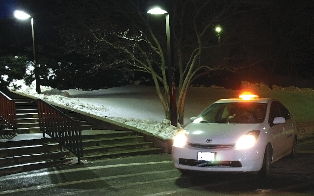
A NU SafeRide car waiting for a student outside Norris

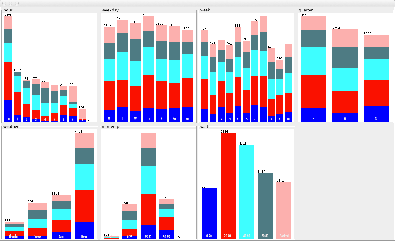
We also looked at which features tend to affect wait times the most and how. The SafeRide executive board could use this information as a tool to decide how many drivers to have on call each night. For example, it is not immediately obvious how bad weather affects SafeRide wait times. It could keep students from going out at all and thus decrease the wait times throughout the night, or it could increase the wait times if students still go out but are more reliant on SafeRides to avoid walking in bad weather. By analyzing these factors, we can develop a set of preferences for the student body that the SafeRide executive board could use to understand when saferide will be busiest.

Our Solution

    Attributes:
  • Hour of the night
  • Week day
  • Week of the quarter
  • Quarter
  • Weather Events*
  • Min Temp*
  • Classifier:
  • Wait time
* Added in second round of testing

We used six attributes to try and predict our classifier. We originally used hour of the night, day of the week, week of the quarter, and the quarter itself. We later added weather events and the minimum recorded temperature for that night. These attributes were used to try and predict our classifier, which was the wait time for a SafeRide at that point in the night. We used these attributes as features in Weka, and were able to test our dataset with a variety of learners. We also sought to try different representations of our dataset, both in discrete and continuous results.

The wait time data was gathered from SafeRide’s twitter, @NUSafeRide. In total there were 10,700 tweets to read from the previous 5 years. We determined the relevance of these tweets through the use of some simple natural language processing. Tweets from @NUSafeRide that are about wait times follow a very simple format, along the lines of “Wait is 45 minutes” or even just “45 mins”. If a tweet followed that or other recognized formats, the time was extracted.

An example tweet from the SafeRide account. We valued this as 40 minutes.

If the wait time couldn’t be recognized, or if it was deemed to be an irrelevant tweet (such as “Happy Holidays!”), then it was not added to the dataset. Once a tweet was established as useful, the timestamp associated with that tweet was used to find other attributes. Hour of the night, day of the week, etc could be directly calculated from the timestamp, while such as week of the quarter or the quarter itself was compared against data gathered from the Office of the Registrar. Finally, weather for the specified time period was downloaded from WeatherUnderground.

Our Testing

Attribute Categorical Continuous
Hour 0,1,2,...,8,9 (0=7pm) numeric
Weekday 0,1,2,...,5,6 (0=M,1=T,etc.) 0 if Su-We; 1 if Thu-Sat
Week of Quarter 0,1,2,...,9,10 numeric
Quarter 0,1,2 (F,W,S) 0,1,2
Weather Events thunderstorm,snow,rain,none 0 if none;1 otherwise
Min Temp <0,0-25,25-50,50-75,>75 numeric
Wait Time 0-20,20-40,40-60,60-80,booked numeric (booked = 90)

We measured success based on whether or not we were able to put our predicted wait time in the same range as the actual wait time. We initially tested many different classifiers and recorded their cross-validated accuracy. Then, we moved forward with the best of these attributes on our training set. For the discrete dataset, we tested to see if our prediction and the actual result fell within the same pre-defined range. For the continuous results, we checked that same set of pre-defined ranges on the actual value and checked it against the predicted value, in order to provide a basis of comparison for the two sets.

Our Results

Discrete:

Overall, the Bayesian algorithms produced the most accurate results. These results were shown to be significant in comparison with the baseline value of the ZeroR Tree that returned an accuracy of 28.3986 %. The best test result from the discrete data was from the HNB algorithm with an accuracy of 39.27% with 359 correctly classified instances. The Lazy Bayesian Rule algorithm also worked well. This had an accuracy of 38.29% with 250 correctly classified instances.

From looking at the data during preprocessing, it appeared some of the attributes had more influence than other on the wait time than others. The wait times did not vary greatly across each day of the week, however it fluctuated greatly depending on the hour of the night.

The discrete data representation. Each chart has bars divided up into the different symbolic representations of each attribute. Those bars are divided by color into the different wait times, which can be referenced in the 'wait' chart.

Continuous:

We were able to produce significant results with our continuous data as well. After converting the data set to reflect numerical values, the ZeroR classifier predicted a value of 42.266 and produced a root mean squared error of 26.2974. When evaluated on our test dataset, it was able to place the data into the correct range 24.316% of the time. Other continuous classifiers were able to perform significantly better on our dataset. The M5P classifier produced the smallest root mean squared error at 24.9658%. The KStar attribute was the most accurate when comparing its prediction to the actual value in our discrete ranges (0-20,20-40, etc). It was able to place the prediction in the same range as the actual value 31.05% of the time, and had a root mean squared error of 25.0113.

Its success may have come from the fact that it uses both decision trees and a series of linear regression equations in order to classify the data. Since some attributes in the data set are better represented as splits rather than a continuous range, creating a preliminary decision tree to separate different examples based on those attributes could have further specified and improved the accuracy of each of the linear regression models. Additionally, the use of an entropy distance measure in the KStar means it it better suited to handle the mix of real-valued and symbolic attributes that made M5P successful.

The continuous data representation. Each bar represents the frequency of each value for that attribute.